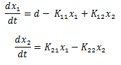
So I have been playing around with a lot of software recently, from starting to write my own operating system (it boots!), learning Unity for making 3D games, and more recently playing around with Google Cardboard and the SDK. The White House released the 2016 budget data so that might call for a machine learning or visualization project. I have been messing around with it but haven't managed to do anything cool with it yet. But today I thought I would mix things up and throw in some math (and MATLAB!). Let's consider a simple model for drug intake, where a substance enters the blood then there is some transfer to the brain. We also assume that some of the drug leaves the bloodstream and the brain at an arbitrary rate.
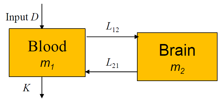
From this we can construct a system of differential equations to describe the system. We can do this by looking at the inputs and outputs of each compartment. But before we do that, we need to add some more details about the parameters.
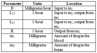
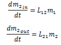
If we focus on the compartment m1, the inputs to the system are on the path D and L21. Since L21 is a rate of exchange measured in 1/hours, the amount of drug moved along it depends on the amount of drug in m2. Therefore, the inputs to the system can be written as:
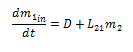
Next, if we consider the outputs, the paths K, and L12 exist. Once again, L12 is a rate dependent on the amount of drugs in m1. So the amount of drugs leaving m1 can be written as L12K, producing the following equations for the outputs of the blood compartment:
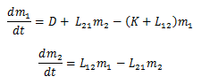
By applying the same analysis to the brain, we can write:
By the mass balance equation:
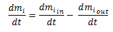
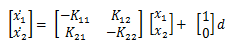
We can combine this into:
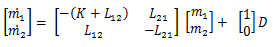
And since I love state space, let’s just transform it:
Both models have the units of Milligrams/hour. The first model states that the change in milligrams of the drug in the bloodstream with respect of time is based on the difference between the inputs and outputs of m1. Drugs enter the bloodstream by either being administered to the patient or returning from the brain to reenter the bloodstream. The drug exits the bloodstream by being taken out of the bloodstream at a rate of K, or being absorbed into the brain. This composes model 1. Model 2 models the change in milligrams of drug in the brain with respect to time. Once again, it is represented as the difference of inputs and outputs. The brain receives the drug through absorbing the drug out of the bloodstream and loses the drug when it returns to the bloodstream.
But in reality, we don’t really think of the amount of drug in a compartment as mass, thus we want to convert the model to concentration. This makes a lot more sense!
If we let  , then
  has the units of milligrams per (liter * hour). So we can define some new parameters:

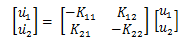
Then we can rewrite the system of equations into the form of:
Or back into state space:
Which we can then find the steady states of!
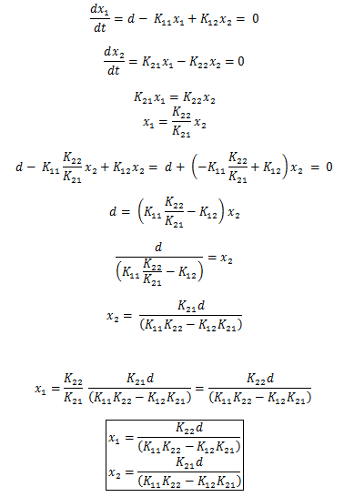
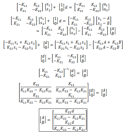
Based on the above math, we can conclude that there is a single steady state that occurs at 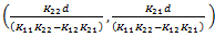 . And based on the nature of the system, we know that K11, K12, K21, K22 > 0.
Furthermore we can gather that d ≥ 0, and with these constraints placed, x1, x2 > 0. Since the numerator cannot go negative (for reasonable values), the only possibility for negativity comes from the denominator. Thus the steady state exists only when K11*K22 > K12*K21. Substituting in for these values based on the prior table gives:
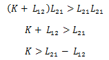
Based on the condition for existence, it is determined that the rate of the drug exiting the bloodstream and the body must be greater than the rate of exchange between the brain and the bloodstream. This condition must be satisfied for the steady state to exist.
Transforming the equations again simplifies the analysis into the stability of the steady states. If we define u1 and u2 as u1 = x1 - A, u2 = x2 - B, then the input, d can be absorbed into A and B. Such that:
Which gives us the state space equations of:
As with any system, we are interested in stability. Therefore we want to show that:
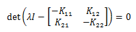
Which gives rise to the polynomial:
The stability can be trivially determined since if K11 * K22 > K12 * K21 then all terms are positive in the characteristic polynomial, which implies stability. However, purely as an exercise and for completeness, we can leverage Routh-Hurwitz Stability Criterion.
When using a Routh-Hurwitz Stability Criterion, the first column must have the same sign. The sign of the first two elements is clearly positive, thus the final element must also be positive for the system to be stable. However, the Routh-Hurwitz Stability Criterion gives one final piece of information that could not be directly concluded from the trivial stability analysis. Since the element in question is the final element in the Criterion, the system will still be stable if K11 * K22 - K12 * K21 = 0, which can be concluded without having to perturb the system and analyze it further. This is only the case since the 0 occurs in the final element of the first column.
Based on this we can conclude that:

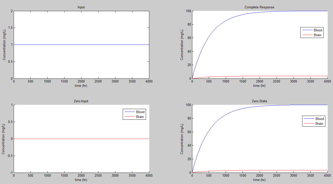
As a sanity check, we can let time go to infinity. The medication in the brain and the blood stabilizes and reaches a constant level as t approaches infinity, when the concentration applied to the subject remains constant. Any adjustments in d will cause the system to asymptotically go to the new steady state value.
Well that's enough math for one day, so let's try to get a simulation of the system in MATLAB working! The code can be found on the Github Repo: 28 Days of Code.
If we set K = 0.01/hr we get the steady state values of 100 for the concentration in mg/L for the blood, and 3.6 for the concentration in the brain.
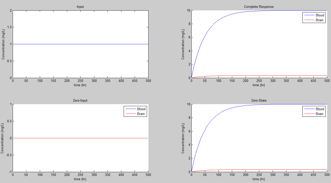
If we set K = 0.1/hr we get the steady state values of 10 for the concentration in mg/L for the blood, and 0.36 for the concentration in the brain.
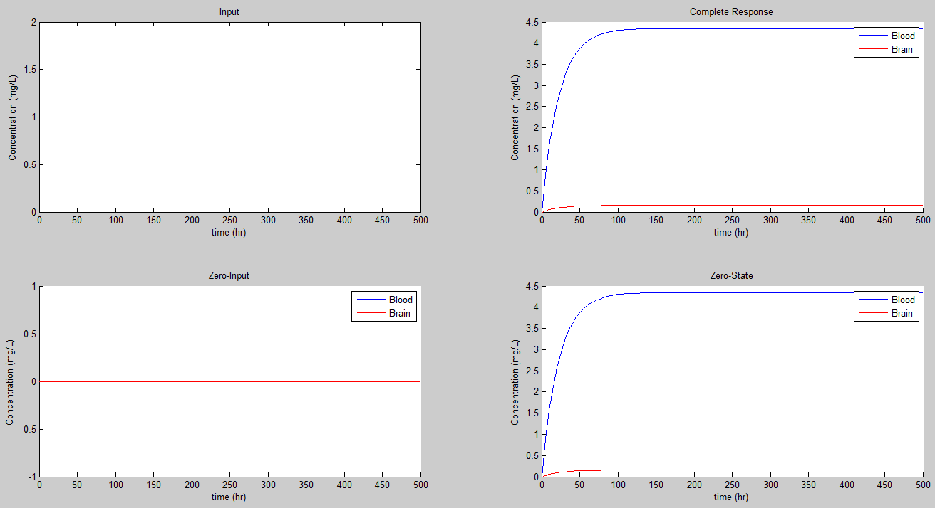
If we set K = 0.23/hr we get the steady state values of 4.3478 for the concentration in mg/L for the blood, and 0.1565 for the concentration in the brain.
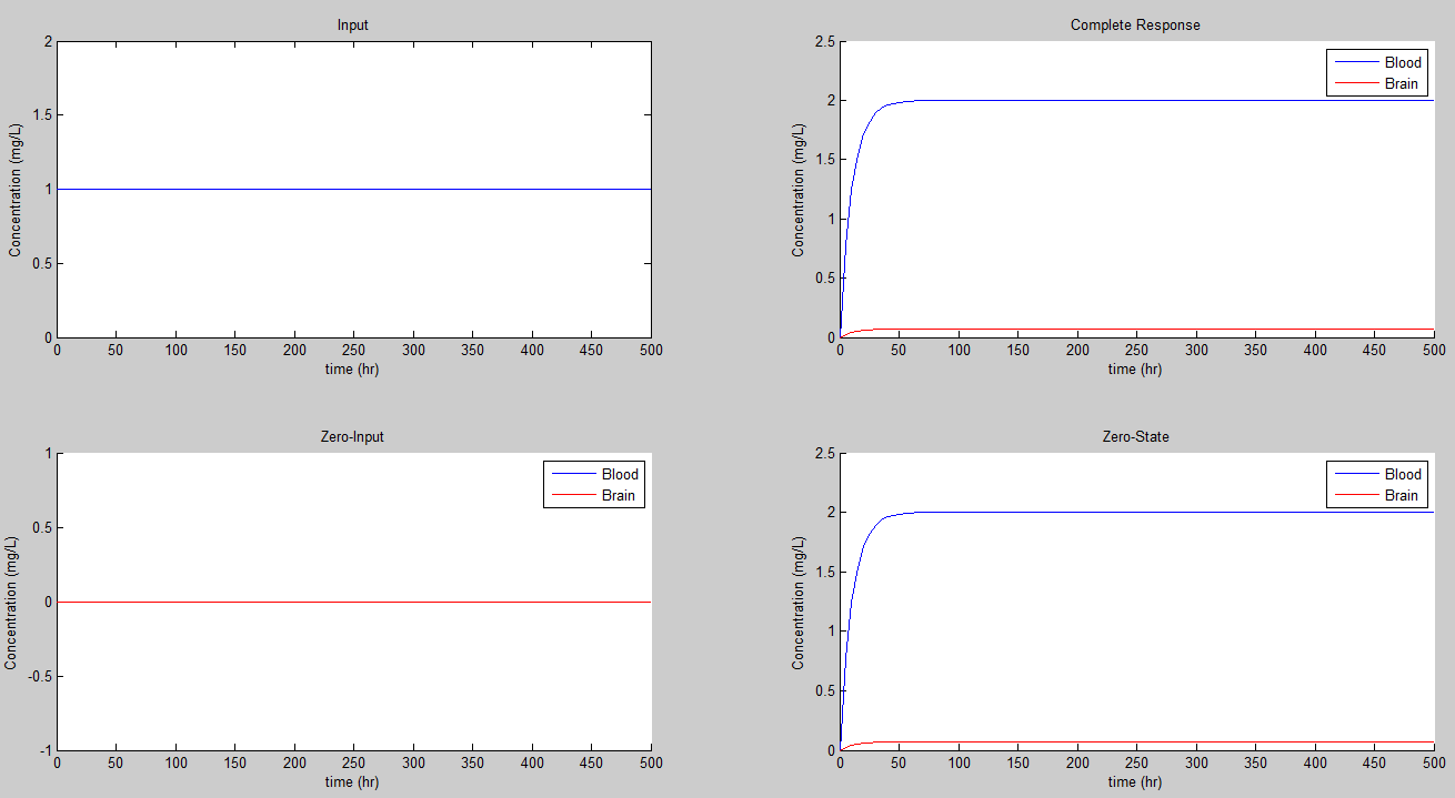
If we set K = 0.5/hr we get the steady state values of 2.0 for the concentration in mg/L for the blood, and 0.072 for the concentration in the brain.
So some conclusions: As K gets smaller, the system becomes less sensitive. It takes longer for the reasonably close to its steady state value, as K gets smaller. Furthermore, as K gets larger, the value of the steady state decreases.
So what happens if we relax the assumptions and no longer apply a constant dosage to a person? What if instead we modeled a pill? This doesn't change the system, just the input so a quick modification to the MATLAB code lets us simulate it. We just have to generate a pulse of amplitude R when 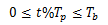 . At any other time, the input is zero, so we have a periodic input relative to Tp.
So if we chose Tp = 2, Tb = 1, R = 1 mg, and simulate from 0 to 30, we get:
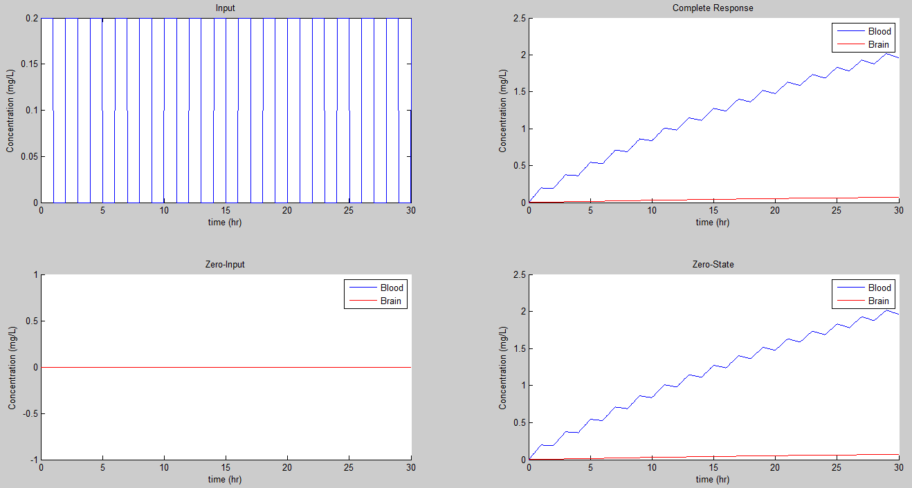
This result is really similar to prior ones but it oscillates. Since the duty cycle is 50%, it just has half the value for steady state.
Now if we let Tp = 2, Tb = 1, R = 1 mg, and simulate from 0 to 120, we get a new plot has similar dynamics to that of the prior one; however, it is a little clearer as to its convergence. It appears to be oscillatory and asymptotically stable for this input. However, for very short periods, the dynamics appear to be slightly chaotic, with an upward trend.
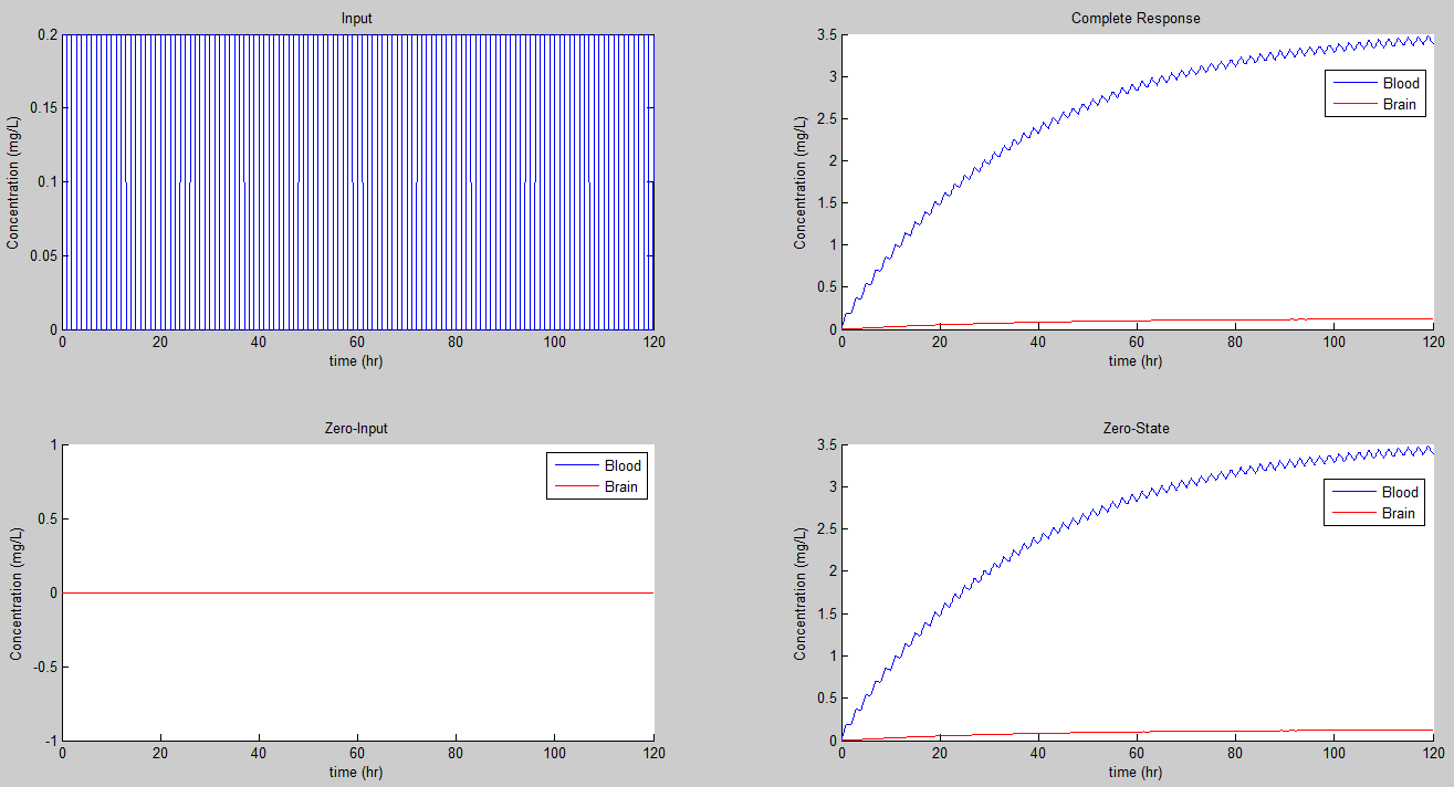
We can play with the values, including for K and produce all kinds of neat results. It is clear that the sensitivity of the periodic dosage is the same as that of the continuous dose medication. However, when switching to a periodic dosage with a 50% duty cycle, the dosage must be twice as large to achieve the same steady state as that of a continuous dosage. We can define the measure B = R*Tb which gives a measure of the encapsulated dosage strength.
Now all the prior results aren't too realistic for a person consuming an encapsulated dose. So we can chose parameters that are more realistic, namely a 4 mg/hr and 1 dose every 24 hours:
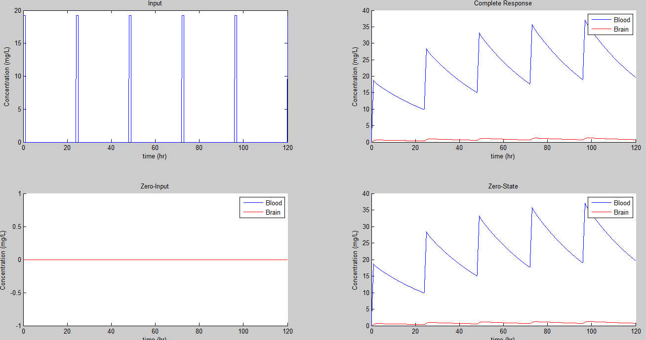
That gives us some very large swings in concentration for both the bloodstream and brain!
So let's try a 4 mg/hr and 1 dose every 6 hours.
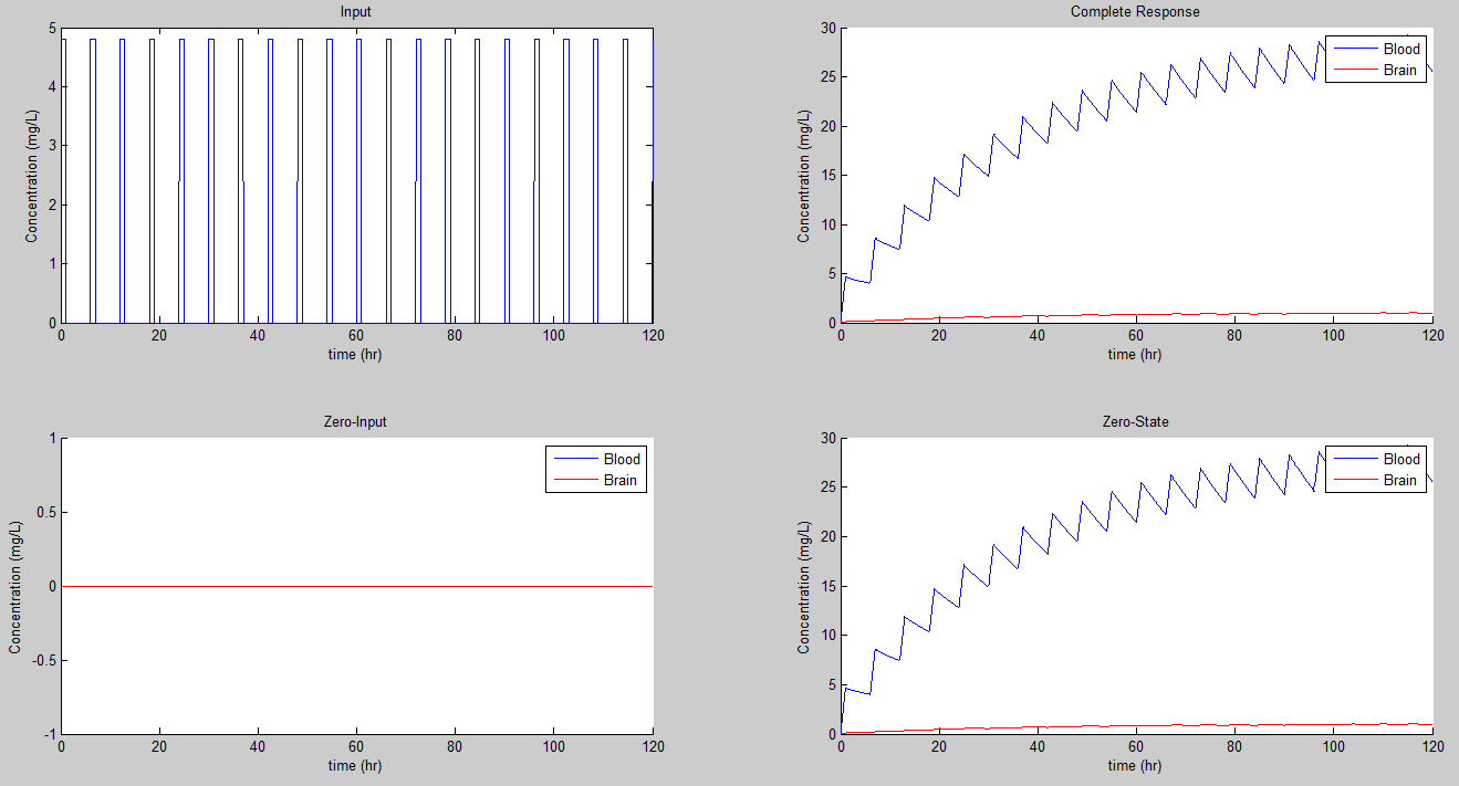
Well we still have plus or minus 5 swings!